Diagnostics

Intra- and inter-chain diagnostics can tell us how well a particular inference algorithm performed on the model. Two common diagnostics are effective sample size, and R-hat.¹

R-hat

$\hat{R}$ is a diagnostic tool that measures the between- and within-chain variances. It is a test that indicates a lack of convergence by comparing the variance between multiple chains to the variance within each chain. If the parameters are successfully exploring the full space for each chain, then $\hat{R}\approx 1$, since the between-chain and within-chain variance should be equal. $\hat{R}$ is calculated from $N$ samples as

$$\hat{R}=\frac{\hat{V}}{W} \\ \hat{V} = \frac{N-1}{N} W + \frac{1}{N} B$$

where $W$ is the within-chain variance, $B$ is the between-chain variance and $\hat{V}$ is the estimate of the posterior variance of the samples. The take-away here is that $\hat{R}$ converges to 1 when each of the chains begins to empirically approximate the same posterior distribution. We do not recommend using inference results if $\hat{R}>1.01$. More information about $\hat{R}$ can be found in the reference ².

Effective Sample Size (ESS)

MCMC samplers do not draw truly independent samples from the target distribution, which means that our samples are correlated. In an ideal situation all samples would be independent, but we do not have that luxury. We can, however, measure the number of effectively independent samples we draw, which is called the effective sample size. You can read more about how this value is calculated in the [2] paper. In brief, it is a measure that combines information from the $\hat{R}$ value with the autocorrelation estimates within the chains.

ESS estimates come in two variants, ess_bulk and ess_tail. The former is the default, but the latter can be useful if you need good estimates of the tails of your posterior distribution. The rule of thumb for ess_bulk is for this value to be greater than 100 per chain on average. Since we ran four chains, we need ess_bulk to be greater than 400 for each parameter. The ess_tail is an estimate for effectively independent samples considering the more extreme values of the posterior. This is not the number of samples that landed in the tails of the posterior, but rather a measure of the number of effectively independent samples if we sampled the tails of the posterior. The rule of thumb for this value is also to be greater than 100 per chain on average.

Diagnostics information with ArviZ

We can use ArviZ, a third-party package for exploratory analysis of Bayesian models, to provide helpful statistics about the result of the inference algorithm, including R-hat and ESS.

To do that, we wrap the result of Bean Machine inference into an InferenceData ArviZ object and use its methods for diagnostic information:

posterior = bm.SingleSiteNewtonianMonteCarlo().infer(
    queries,
    observations,
    num_samples,
    num_chains,
)

import arviz as az
inference_data = az.convert_to_inference_data(posterior.samples)
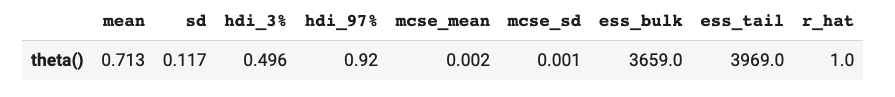
az.summary(inference_data)

which in a notebook outputs something like:

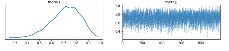
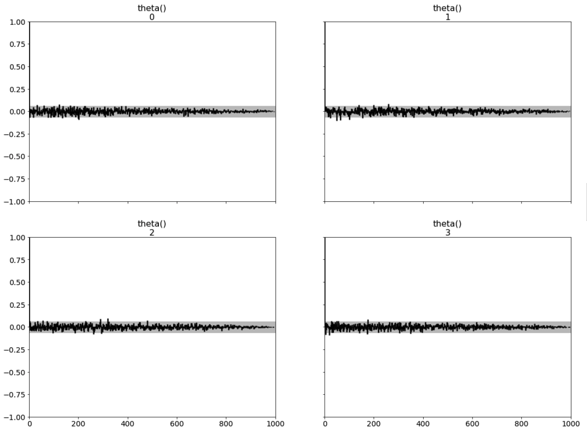
ArviZ provides many other analysis tools, including trace and autocorrelation plots:

az.plot_trace(inference_data);

az.plot_autocorr(inference_data, combined=False, max_lag=1000, grid=(2,2));

¹ Stan Reference Manual. https://mc-stan.org/docs/2_18/reference-manual/effective-sample-size-section.html

² Vehtari A, Gelman A, Simpson D, Carpenter B, Bürkner PC (2021) Rank-Normalization, Folding, and Localization: An Improved $\hat{R}$ for Assessing Convergence of MCMC (with Discussion). Bayesian Analysis 16(2) 667–718. doi: 10.1214/20-BA1221.